rkstiff

Exponential time–differencing (ETD) and integrating factor (IF) Runge–Kutta solvers for stiff semi-linear PDEs:

$u_t = L u + \mathrm{NL}(u)$

• Fast, adaptive, and pure Python (NumPy/SciPy only)
• Embedded error control, logging, and flexible operator support
• Designed for spectral methods and diagonalizable systems

Tested: Python 3.9–3.13 | Dependencies: NumPy, SciPy | Optional: matplotlib, jupyter, pytest

Docs: rkstiff.readthedocs.io

---

Features

• Adaptive ETD/IF Runge–Kutta solvers: ETD35, ETD34, IF34, IF45DP (embedded error control)
• Fixed-step solvers: ETD4, ETD5, IF4
• Operator flexibility: Diagonal or full matrix (spectral/finite-difference)
• Spectral methods: Fourier/Chebyshev support
• Configurable error control: SolverConfig for tolerances, safety factors
• Logging: Per-solver logging, adjustable verbosity
• Lightweight API: Pass a linear operator array and a callable nonlinear function
• Utility modules: Grids, spectral derivatives, transforms, models, logging helpers

Supported equations: Nonlinear Schrödinger, Kuramoto–Sivashinsky, Korteweg–de Vries, Burgers, Allen–Cahn, Sine–Gordon

---

Installation

pip (recommended):

python -m pip install rkstiff

conda-forge:

conda create -n rkstiff-env -c conda-forge rkstiff
conda activate rkstiff-env

From source:

git clone https://github.com/whalenpt/rkstiff.git
cd rkstiff
python -m pip install .

Extras:

# demos: matplotlib + jupyter; tests: pytest
python -m pip install "rkstiff[demo]"
python -m pip install "rkstiff[test]"

---

Quickstart Example (Kuramoto–Sivashinsky)

import numpy as np
from rkstiff import grids, if34

# Real-valued grid for rfft
n = 1024
a, b = 0.0, 32.0 * np.pi
x, kx = grids.construct_x_kx_rfft(n, a, b)

# Linear operator in Fourier space
lin_op = kx**2 * (1 - kx**2)

# Nonlinear term: -F{ u * u_x }
def nl_func(u_fft):
    u = np.fft.irfft(u_fft)
    ux = np.fft.irfft(1j * kx * u_fft)
    return -np.fft.rfft(u * ux)

# Initial condition in real space → Fourier space
u0 = np.cos(x / 16) * (1.0 + np.sin(x / 16))
u0_fft = np.fft.rfft(u0)

solver = if34.IF34(lin_op=lin_op, nl_func=nl_func)
uf_fft = solver.evolve(u0_fft, t0=0.0, tf=50.0, store_freq=20)

# Convert stored Fourier snapshots back to real space
U = np.array([np.fft.irfft(s) for s in solver.u])  # shape: (num_snaps, n)
t = np.array(solver.t)

solver.u and solver.t store snapshots every store_freq internal steps; evolve returns the final state.

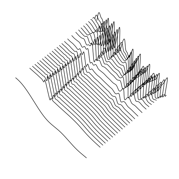
Kuramoto–Sivashinsky chaotic field propagation using IF34.

💡 More examples:
Several fully runnable Jupyter notebooks are included in the demos/ folder.
Each notebook illustrates solver usage, adaptive-step control, and visualization for different PDEs
(e.g., Kuramoto–Sivashinsky, NLS, and Allen–Cahn).
To try them:

python -m pip install "rkstiff[demo]"
jupyter notebook demos/

---

API Overview

Solver Classes

Solver	Module	Order (embedded)	Adaptive	Notes
ETD35	etd35	5 (3)	✅	Best for diagonalized systems
ETD34	etd34	4 (3)	✅	Krogstad 4th order
IF34	if34	4 (3)	✅	Integrating factor
IF45DP	if45dp	5 (4)	✅	Dormand–Prince IF
ETD4	etd4	4 (–)	❌	Krogstad fixed-step
ETD5	etd5	5 (–)	❌	Same base as ETD35
IF4	if4	4 (–)	❌	Fixed-step IF

Constructor Signature (Adaptive Classes)

Solver(lin_op: np.ndarray, nl_func: Callable[[np.ndarray], np.ndarray], config: SolverConfig = ..., loglevel: str = ...)

• lin_op: array shaped like u, typically diagonal entries in the working basis
• nl_func(u): returns nonlinear term in same basis
• config: error control and adaptivity (optional; defaults to SolverConfig())
• loglevel: logging verbosity (optional; defaults to "INFO")

---

Configuration & Logging

Adaptive Error Control

Configure embedded error estimation and adaptive step control via SolverConfig:

from rkstiff.if34 import IF34
from rkstiff.solveras import SolverConfig

config = SolverConfig(epsilon=1e-5, incr_f=1.2, decr_f=0.8, safety_f=0.9)
solver = IF34(lin_op, nl_func, config=config, loglevel="INFO")

Parameter notes (typical meanings):

• epsilon: target local error tolerance for the embedded pair.
• safety_f: safety factor applied to proposed step-size updates.
• incr_f / decr_f: bounds on how much dt may grow/shrink on accept/reject.
• (Implementation-specific fields may exist; see docs for full list and defaults.)

Logging

Set logging level per solver:

solver = IF34(lin_op, nl_func, loglevel="DEBUG")

---

Utility Modules

• grids: Grid and wavenumber construction for FFT/RFFT/Chebyshev
• derivatives: Spectral differentiation (FFT, RFFT, Chebyshev)
• transforms: Basis transforms
• models: Example PDEs
• util.loghelper: Logging setup and control

---

Usage Tips

• For spectral methods, pass lin_op in Fourier space and implement nl_func in that same space
• For diagonalizable systems, pre-diagonalize once and reuse that basis
• ETD methods may precompute φ-functions; reuse the solver instance for speed
• Storage: solver.u and solver.t hold snapshots; control frequency with store_freq

---

Testing & Coverage

Run tests and view coverage:

python -m pip install "rkstiff[test]"
pytest

---

Citation

If you use rkstiff in academic work, please cite:

P. Whalen, M. Brio, J.V. Moloney, Exponential time-differencing with embedded Runge–Kutta adaptive step control, Journal of Computational Physics 280 (2015) 579–601. DOI: 10.1016/j.jcp.2014.09.038

@article{WhalenBrioMoloney2015,
  title   = {Exponential time-differencing with embedded Runge--Kutta adaptive step control},
  author  = {Whalen, P. and Brio, M. and Moloney, J. V.},
  journal = {Journal of Computational Physics},
  volume  = {280},
  pages   = {579--601},
  year    = {2015},
  doi     = {10.1016/j.jcp.2014.09.038}
}

---

License

MIT — see LICENSE for details.

Contact

Patrick Whalen — [email protected]