E2

This is the second excercise.

Making a directory

mkdir -p kata/data

cd kata/data

Starting a screen

screen -S kata

Saving data

cp /data-shared/vcf_examples/luscinia_vars.vcf.gz .

Extracting information about DP of the whole genome

< /data-shared/vcf_examples/luscinia_vars.vcf.gz zcat | egrep -o 'DP=[^;]*' | sed 's/DP=//' > g.csv

Saving your extracted data from the whole genome

Now you have to run this command on your "home" machine. Katerinka$ scp [email protected]:projects/kata/g.csv .

Now, for extracting DP for each chromosome separately, I decided to create a function

chrfun() { zcat | grep -v '^#' | grep $1| egrep -o 'DP=[^;]*' | sed 's/DP=//' > $2.csv ;}

$1 is the name of the chromosome, $2 is the under which I want to safe my file. Then, we can run the function on the data, we are interested in.

< /data-shared/vcf_examples/luscinia_vars_flags.vcf.gz chrfun '^chrZ\s' zet

Again, we have to save to our local disk

scp [email protected]:projects/kata/zet.csv .

In R studio – start by setting a working directory

setwd("~/Desktop/PřF UK/UNIX"

Loading my file

datag <- read.csv("g.csv", col.names = "DP")

Plotting a graph (histogram) for whole genome

datag %>% ggplot(aes(DP)) + geom_histogram() + scale_y_log10()

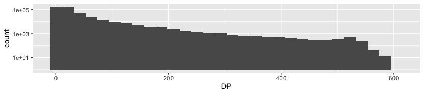
In this graph we can see how many reads (y) of a certain length (x) we can find after sequencing. There is a big varienty, taking into account, that y axis is logarithmical.

For separate chromosome (I took Z as an example)

dataz <- read.csv("zet.csv", col.names = "DP")

Plotting a graph (histogram) for one separate chromosome (Z)

dataz %>% ggplot(aes(DP)) + geom_histogram() + scale_y_log10()

Trying to find another solution

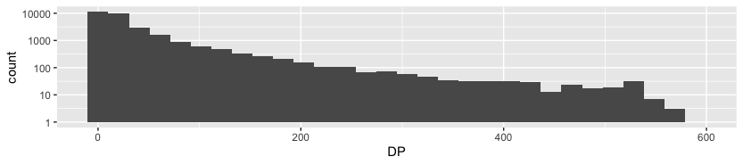
Since my solution shown above is plotting DP against its counts (so basically showing distribution of occurences of some DP), I decided to plot it against its loci, which can be quite useful (it helps us to know, which part of choromosome is being amplified most often).

Secondly, for one separate chromosome (in this case chromosome 1)

Working in the same directory, let's remove headers and extract data only for the chromosome of interest

< /data-shared/vcf_examples/luscinia_vars_flags.vcf.gz zcat | grep -v '^#' | grep -e 'chr1\s' > data/nh.vcf

Now we can extract two columns into two separate steps and we have to save them as two separate files

(I tried to do it into one step, but it obviously doesn't work. I can't remove the column and then try to filter it...)

IN=data/nh.vcf <$IN cut -f2 > data/POS.tsv <$IN egrep -o 'DP=[^;]*' | sed 's/DP=//' > data/DP.tsv

Let's merge two columns of interest together in one single file (for future use in R)

paste data/POS.tsv data/DP.tsv > ch1.tsv

And open it from our local disk

scp [email protected]:projects/kata/ch1.tsv .

Plotting in R

setwd("~/Desktop/PřF UK/UNIX")

dat <- read_tsv("ch1.tsv", col_names=c("POS", "DP"))

dat %>% ggplot(aes(POS, DP)) + geom_line()

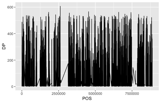
In the plot (having read depth on y and position of loci on x) we can see, that there are some gaps i reads – almost looks like some deletion event.

How will it look like for the whole genome? Same, just without column extraction according to the chromosome

First delete headers

< /data-shared/vcf_examples/luscinia_vars_flags.vcf.gz zcat | grep -v '^#' > data/nhg.vcf

Here comes the column extraction

IN=data/nhg.vcf <$IN cut -f2 > data/POSg.tsv <$IN egrep -o 'DP=[^;]*' | sed 's/DP=//' > data/DPg.tsv

Let's merge two columns of interest together in one single file (for future use in R)

paste data/POSg.tsv data/DPg.tsv > gg.tsv

Open in it on your local disk

scp [email protected]:projects/kata/gg.tsv .

And plotting graph in R (in the same wd)

datg <- read_tsv("gg.tsv", col_names=c("POS", "DP"))

dat %>% ggplot(aes(POS, DP)) + geom_line()

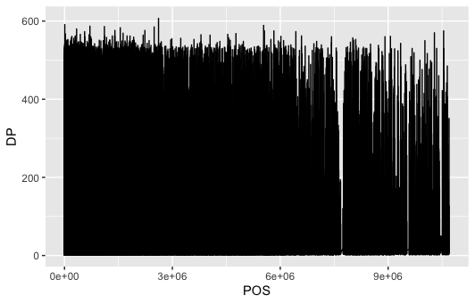
We can see, that the genome isn't covered in some portions.