JobShopLib

JobShopLib is a Python package for creating, solving, and visualizing job shop scheduling problems.

It provides solvers based on:

• Graph neural networks (Gymnasium environment)
• Dispatching rules
• Simulated annealing
• Constraint programming (CP-SAT from Google OR-Tools)

It also includes utilities for:

• Load benchmark instances
• Generating random problems
• Gantt charts
• Disjunctive graphs (and any variant)
• Training a GNN-based dispatcher using reinforcement learning or imitation learning

It supports:

• Multi-machine operations
• Release dates
• Deadlines and due dates

JobShopLib's design is intended to be modular and easy-to-use:

import matplotlib.pyplot as plt
plt.style.use("ggplot")

from job_shop_lib import JobShopInstance, Operation
from job_shop_lib.benchmarking import load_benchmark_instance
from job_shop_lib.generation import GeneralInstanceGenerator
from job_shop_lib.constraint_programming import ORToolsSolver
from job_shop_lib.visualization import plot_gantt_chart, create_gif, plot_gantt_chart_wrapper
from job_shop_lib.dispatching import DispatchingRuleSolver

# Create your own instance manually,
job_1 = [Operation(machines=0, duration=1), Operation(1, 1), Operation(2, 7)]
job_2 = [Operation(1, 5), Operation(2, 1), Operation(0, 1)]
job_3 = [Operation(2, 1), Operation(0, 3), Operation(1, 2)]
jobs = [job_1, job_2, job_3]
instance = JobShopInstance(jobs)

# load a popular benchmark instance,
ft06 = load_benchmark_instance("ft06")

# or generate a random one.
generator = GeneralInstanceGenerator(
    duration_range=(5, 10), seed=42, num_jobs=5, num_machines=5
)
random_instance = generator.generate()

# Solve it using constraint programming,
solver = ORToolsSolver(max_time_in_seconds=10)
ft06_schedule = solver(ft06)

# Visualize the solution as a Gantt chart,
fig, ax = plot_gantt_chart(ft06_schedule)
plt.show()

# or visualize how the solution is built step by step using a dispatching rule.
mwkr_solver = DispatchingRuleSolver("most_work_remaining")
plt.style.use("ggplot")
plot_function = plot_gantt_chart_wrapper(
    title="Solution with Most Work Remaining Rule"
)
create_gif(  # Creates the gif above
    gif_path="ft06_optimized.gif",
    instance=ft06,
    solver=mwkr_solver,
    plot_function=plot_function,
    fps=4,
)

Installing 📦

pip install job-shop-lib

Quick Start 🚀

Create a Job Shop Instance

You can create a JobShopInstance by defining the jobs and operations. An operation is defined by the machine(s) it is processed on and the duration (processing time).

from job_shop_lib import JobShopInstance, Operation


job_1 = [Operation(machines=0, duration=1), Operation(1, 1), Operation(2, 7)]
job_2 = [Operation(1, 5), Operation(2, 1), Operation(0, 1)]
job_3 = [Operation(2, 1), Operation(0, 3), Operation(1, 2)]

jobs = [job_1, job_2, job_3]

instance = JobShopInstance(
    jobs,
    name="Example",
    # Any extra parameters are stored inside the
    # metadata attribute as a dictionary:
    lower_bound=7,
)

Load a Benchmark Instance

You can load a benchmark instance from the library:

from job_shop_lib.benchmarking import load_benchmark_instance

ft06 = load_benchmark_instance("ft06")

The module benchmarking contains functions to load the instances from the file and return them as JobShopInstance objects without having to download them manually.

The contributions to this benchmark dataset are as follows:

• abz5-9: by Adams et al. (1988).

• ft06, ft10, ft20: by Fisher and Thompson (1963).

• la01-40: by Lawrence (1984)

• orb01-10: by Applegate and Cook (1991).

• swv01-20: by Storer et al. (1992).

• yn1-4: by Yamada and Nakano (1992).

• ta01-80: by Taillard (1993).

The metadata from these instances has been updated using data from: https://github.com/thomasWeise/jsspInstancesAndResults

>>> ft06.metadata
{'optimum': 55,
 'upper_bound': 55,
 'lower_bound': 55,
 'reference': "J.F. Muth, G.L. Thompson. 'Industrial scheduling.', Englewood Cliffs, NJ, Prentice-Hall, 1963."}

Generate a Random Instance

You can also generate a random instance with the GeneralInstanceGenerator class.

from job_shop_lib.generation import GeneralInstanceGenerator

generator = GeneralInstanceGenerator(
    duration_range=(5, 10), seed=42, num_jobs=5, num_machines=5
)
random_instance = generator.generate()

This class can also work as an iterator to generate multiple instances:

generator = GeneralInstanceGenerator(iteration_limit=100, seed=42)
instances = []
for instance in generator:
    instances.append(instance)

# Or simply:
instances = list(generator)

Solve an Instance with the OR-Tools' Constraint-Programming SAT Solver

Every solver is a Callable that receives a JobShopInstance and returns a Schedule object.

import matplotlib.pyplot as plt

from job_shop_lib.constraint_programming import ORToolsSolver
from job_shop_lib.visualization import plot_gantt_chart

solver = ORToolsSolver(max_time_in_seconds=10)
ft06_schedule = solver(ft06)

fig, ax = plot_gantt_chart(ft06_schedule)
plt.show()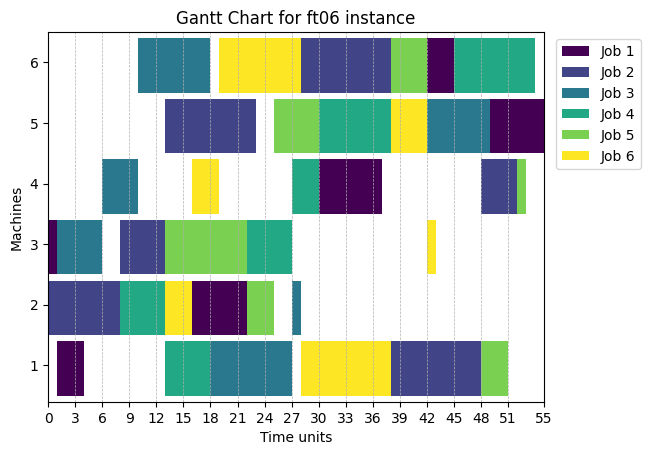

Solve an Instance with a Dispatching Rule Solver

A dispatching rule is a heuristic guideline used to prioritize and sequence jobs on various machines. Supported dispatching rules are (although you can also create your own):

class DispatchingRule(str, Enum):
    SHORTEST_PROCESSING_TIME = "shortest_processing_time"
    LARGEST_PROCESSING_TIME = "largest_processing_time"
    FIRST_COME_FIRST_SERVED = "first_come_first_served"
    MOST_WORK_REMAINING = "most_work_remaining"
    MOST_OPERATION_REMAINING = "most_operation_remaining"
    RANDOM = "random"

We can visualize the solution with a DispatchingRuleSolver as a gif:

from job_shop_lib.visualization import create_gif, plot_gantt_chart_wrapper
from job_shop_lib.dispatching import DispatchingRuleSolver, DispatchingRule

plt.style.use("ggplot")

mwkr_solver = DispatchingRuleSolver("most_work_remaining")
plot_function = plot_gantt_chart_wrapper(
    title="Solution with Most Work Remaining Rule"
)
create_gif(
    gif_path="ft06_optimized.gif",
    instance=ft06,
    solver=mwkr_solver,
    plot_function=plot_function,
    fps=4,
)

The dashed red line represents the current time step, which is computed as the earliest time when the next operation can start.

Tip

You can change the style of the gantt chart with plt.style.use("name-of-the-style"). Personally, I consider the ggplot style to be the cleanest.

Representing Instances as Graphs

One of the main purposes of this library is to provide an easy way to encode instances as graphs. This can be very useful, not only for visualization purposes but also for developing graph neural network-based algorithms.

Disjunctive Graph

from job_shop_lib.visualization import plot_disjunctive_graph

fig = plot_disjunctive_graph(
    instance,
    figsize=(6, 4),
    draw_disjunctive_edges="single_edge",
    disjunctive_edges_additional_params={
        "arrowstyle": "<|-|>",
        "connectionstyle": "arc3,rad=0.15",
    },
)
plt.show()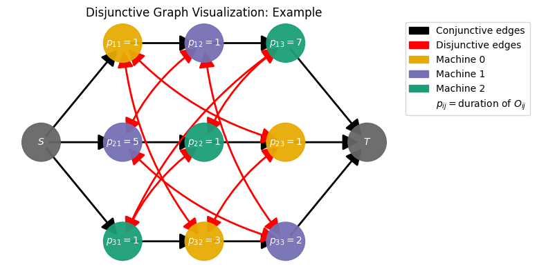

Tip

Installing the optional dependency PyGraphViz is recommended.

Resource-Task Graph

Introduced in the paper "ScheduleNet: Learn to solve multi-agent scheduling problems with reinforcement learning" by Park et al. (2021), the resource-task graph (orginally named "agent-task graph") is a graph that represents the scheduling problem as a multi-agent reinforcement learning problem.

In contrast to the disjunctive graph, instead of connecting operations that share the same resources directly by disjunctive edges, operation nodes are connected with machine ones.

All machine nodes are connected between them, and all operation nodes from the same job are connected by non-directed edges too.

from job_shop_lib.graphs import (
    build_complete_resource_task_graph,
    build_resource_task_graph_with_jobs,
    build_resource_task_graph,
)
from job_shop_lib.visualization import plot_resource_task_graph

resource_task_graph = build_resource_task_graph(instance)

fig = plot_resource_task_graph(resource_task_graph)
plt.show()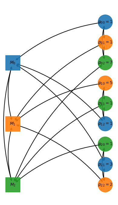

---

The library generalizes this graph by allowing the addition of job nodes and a global one (see build_resource_task_graph_with_jobs and build_resource_task_graph).

Gymnasium Environments

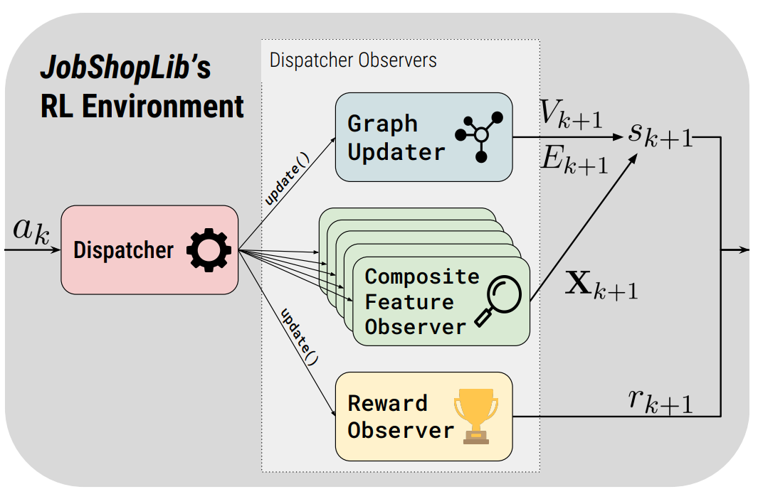
The SingleJobShopGraphEnv allows to learn from a single job shop instance, while the MultiJobShopGraphEnv generates a new instance at each reset. For an in-depth explanation of the environments see chapter 7 of my Bachelor's thesis.

from IPython.display import clear_output

from job_shop_lib.reinforcement_learning import (
    # MakespanReward,
    SingleJobShopGraphEnv,
    ObservationSpaceKey,
    IdleTimeReward,
    ObservationDict,
)
from job_shop_lib.dispatching.feature_observers import (
    FeatureObserverType,
    FeatureType,
)
from job_shop_lib.dispatching import DispatcherObserverConfig


instance = load_benchmark_instance("ft06")
job_shop_graph = build_disjunctive_graph(instance)
feature_observer_configs = [
    DispatcherObserverConfig(
        FeatureObserverType.IS_READY,
        kwargs={"feature_types": [FeatureType.JOBS]},
    )
]

env = SingleJobShopGraphEnv(
    job_shop_graph=job_shop_graph,
    feature_observer_configs=feature_observer_configs,
    reward_function_config=DispatcherObserverConfig(IdleTimeReward),
    render_mode="human",  # Try "save_video"
    render_config={
        "video_config": {"fps": 4}
    }
)


def random_action(observation: ObservationDict) -> tuple[int, int]:
    ready_jobs = []
    for job_id, is_ready in enumerate(
        observation[ObservationSpaceKey.JOBS.value].ravel()
    ):
        if is_ready == 1.0:
            ready_jobs.append(job_id)

    job_id = random.choice(ready_jobs)
    machine_id = -1  # We can use -1 if each operation can only be scheduled
    # on one machine.
    return (job_id, machine_id)


done = False
obs, _ = env.reset()
while not done:
    action = random_action(obs)
    obs, reward, done, *_ = env.step(action)
    if env.render_mode == "human":
        env.render()
        clear_output(wait=True)

if env.render_mode == "save_video" or env.render_mode == "save_gif":
    env.render()

Contributing 🤝

Any contribution is welcome, whether it's a small bug or documentation fix or a new feature! See the CONTRIBUTING.md file for details on how to contribute to this project.

License 📜

This project is licensed under the MIT License - see the LICENSE file for details.

Publication 📜

For an in-depth explanation of the library (v1.0.0), including its design, features, reinforcement learning environments, and some experiments, please refer to https://www.arxiv.org/abs/2506.13781.

You can also cite the library using the following BibTeX entry:

@misc{arino2025jobshoplib,
      title={Solving the Job Shop Scheduling Problem with Graph Neural Networks: A Customizable Reinforcement Learning Environment}, 
      author={Pablo Ariño Fernández},
      year={2025},
      eprint={2506.13781},
      archivePrefix={arXiv},
      primaryClass={cs.LG},
      url={https://arxiv.org/abs/2506.13781}, 
}

References 📚

• Peter J. M. van Laarhoven, Emile H. L. Aarts, Jan Karel Lenstra, (1992) Job Shop Scheduling by Simulated Annealing. Operations Research 40(1):113-125.

• J. Adams, E. Balas, and D. Zawack, "The shifting bottleneck procedure for job shop scheduling," Management Science, vol. 34, no. 3, pp. 391–401, 1988.

• J.F. Muth and G.L. Thompson, Industrial scheduling. Englewood Cliffs, NJ: Prentice-Hall, 1963.

• S. Lawrence, "Resource constrained project scheduling: An experimental investigation of heuristic scheduling techniques (Supplement)," Carnegie-Mellon University, Graduate School of Industrial Administration, Pittsburgh, Pennsylvania, 1984.

• D. Applegate and W. Cook, "A computational study of job-shop scheduling," ORSA Journal on Computer, vol. 3, no. 2, pp. 149–156, 1991.

• R.H. Storer, S.D. Wu, and R. Vaccari, "New search spaces for sequencing problems with applications to job-shop scheduling," Management Science, vol. 38, no. 10, pp. 1495–1509, 1992.

• T. Yamada and R. Nakano, "A genetic algorithm applicable to large-scale job-shop problems," in Proceedings of the Second International Workshop on Parallel Problem Solving from Nature (PPSN'2), Brussels, Belgium, pp. 281–290, 1992.

• E. Taillard, "Benchmarks for basic scheduling problems," European Journal of Operational Research, vol. 64, no. 2, pp. 278–285, 1993.

• Park, Junyoung, Sanjar Bakhtiyar, and Jinkyoo Park. "ScheduleNet: Learn to solve multi-agent scheduling problems with reinforcement learning." arXiv preprint arXiv:2106.03051, 2021.